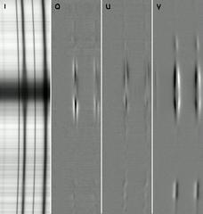
 The Spectral-polarimeter (SP) obtains line profiles of two magnetically sensitive Fe lines at 630.15 and 630.25 nm and nearby contiuum, using a 0.16"×164" slit. Spectra are exposed and read out continuously 16 times per rotation of the polarization modulator, and the raw spectra are added and subtracted onboard in real time to demodulate, generating Stokes IQUV spectral images. Two spectra are simultaneously taken in orthogonal linear polarizations. When combined in data analysis after downlink, spurious polarization due to any residual image jitter or solar evolution is greatly reduced. The slit can move to map a finite area, up to the full 320" wide FOV.
| Field of view along slit | 164" (north-south direction) |
| Spatial scan range | ±164" |
| Slit width | 0.16" |
| Spectral coverage | 630.08nm - 630.32nm |
| Spectral resolution / sampling | 30mÅ / 21.5mÅ |
| Measurement of polarization | Stokes I,Q,U,V simultaneously with dual beams (orthogonal linear components) |
| Polarization signal to noise | 103 (with normal mapping) |
The SP is flexible in mapping observing regions, allowing one to perform suitable observations depending on science objectives (Table 2). The SP only has a few modes of operation: Normal Map, Fast Map, Dynamics, and Deep Magnetogram. The Normal Map mode produces polarimetric accuracy of 0.1% with the spatial sampling of 0.16"×0.16". It takes 83 min to scan a 160" wide area: enough to cover a moderate-sized active region. By reducing the scanning size, the cadence becomes faster (50 sec for mapping of 1.6" wide area), which would be useful for studying dynamics of small magnetic features. The Fast Map mode of observation can provide 30-min cadence for the 160" wide scanning with polarimetric accuracy of 0.1% but 0.32" resolution. The Dynamics mode of observation provides higher cadence (18 sec for 1.6" wide area) with 0.16" resolution, although at lower polarimetric accuracy. In Deep Magnetogram mode, photons may be accumulated over many rotations of the polarization modulator, as long as the data doesn't overflow the summing registers. This allows one to achieve a very high polarization accuracy in very quiet regions, at the expense of time resolution.
| Normal map | Time per position | 4.8 sec (3 rotations of waveplate) |
|---|---|---|
| FOV along slit | 164" | |
| Sampling along slit | 0.16" | |
| Slit-scan sampling | 0.16" | |
| Polarimetric S/N | 103 | |
| Data size | 918k pixels in 4.8 sec (191k pixel/s) | |
| Time for map area | 50sec for 1.6" wide 83min for 160" wide |
|
| Fast map | Time per position | 3.2 sec (one rotation for 1st slit position and another rotation for 2nd slit position) |
| FOV along slit | 164" | |
| Sampling along slit | 0.32" | |
| Slit-scan sampling | 0.32" | |
| Polarimetric S/N | 103 | |
| Data size | 459k pixels in 3.6 sec (127k pixel/s) | |
| Time for map area | 18sec for 1.6" wide 30min for 160" wide |
|
| Dynamics | Time per position | 1.6 sec (one rotation of waveplate) |
| FOV along slit | 32" | |
| Sampling along slit | 0.16" | |
| Slit-scan sampling | 0.16" | |
| Polarimetric S/N | 580 | |
| Data size | 179k pixels in 1.6 sec (120k pixel/s) | |
| Time for map area | 18sec for 1.6" wide | |
| Deep magnetogram | Time per position | many rotations (up to 8 rotations) |
| FOV along slit | 164" | |
| Sampling along slit | 0.16" | |
| Slit-scan sampling | 0.16" | |
| Polarimetric S/N | >103 |